User guide¶

The following chapters describe the usage for the GUI. For details on the simple-plotter file format and the CLI tool see the Advanced usage chapter.

The screen shots in this user guide are taken from the Android port simple-plotter4a, but all features are available in the Qt-GUI as well.

Overview¶

simple-plotter’s main purpose is to serve as graphical calculator for creating 2D plots of x,y-functions and provides following features:

define functions in python/NumPy syntax
it gives access to all NumPy methods
projects can be saved and restored
projects can also be exported to python scripts
constants and curve set parameters can be defined
axes can be changed to logarithmic scale
plot annotations (e.g. plot title and labels) are automatically generated

Defining an equation¶

To define an equation you must specify the values of the three input fields on the top:

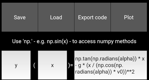
Function name (mandatory): The function name (e.g. ‘f’ or ‘y’) will be displayed on the y-axis of the plot. It has no further effect on the calculation, so it is really just a label for the y-axis.
Variable name (mandatory): The name of the variable (e.g. ‘x’), which will be displayed on the x-axis of the plot. In contrast to the function name this is not just used for the label. This value must match the variable in the equation field.
Equation (mandatory): Here you can define the equation (e.g. 3*x**2 + 2*x + 5). As mentioned above you will have to define a variable name in the variable field. Note, that your equation must be formatted in valid python syntax. If you are not familiar with python syntax have a look at the Using Python as as a Calculator chapter in the official python tutorial. You can additionally use any function/constants of the NumPy package by prepending a ‘np.’ - e.g. your equation could be: 3 * np.sin(x) + 2 * np.cos(x / np.pi)

Creating a plot¶

If you have entered the equation definition correctly just press the ‘Plot’ button and a graph will be rendered for your equation. You can alter the plot appearance in ‘Plot settings’ section.

Adjust the plot appearance¶

The plot appearance can be altered in the ‘Plot settings’ section.

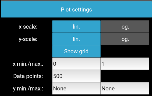
You can change following parameters:

x-scale: Sets the x-axis either to linear scale (default) or to logarithmic scale. Note, that for logarithmic scale only values greater than 0 can be displayed.
y-scale: Sets the y-axis either to linear scale (default) or to logarithmic scale. Note, that for logarithmic scale only values greater than 0 can be displayed.
show grid: Shows or hides the grid
x-min./max. (mandatory): Defines the bounds of x-axis. Both values are mandatory inputs. Note, that if you set the x-axis to logarithmic scale negative values will be ignored - i.e. the bounds will be re-calculated automatically.
Data points (mandatory): Specifies the number of data points used to calculate the x,y-values for each curve. Increase this value to create smoother curves.
y-min./max. (optional): Defines the bounds of x-axis. Both values are optional. If not defined they will be adjusted to fit all curve data points into the graph. Note, that if you set the x-axis to logarithmic scale negative values will be ignored - i.e. the bounds will be re-calculated automatically.

Constants¶

simple-plotter allows you to extend your equation with constants - e.g. ‘a*x**2 + b*x + c’, where a, b and c are constants.

You can define two different types of constants:

multiple single valued (‘normal’) constants - e.g. g = 9.81

one set constant to create curve sets - i.e. the set constant takes multiple values (see next chapter)

The ‘normal’ constants can be defined in the ‘Constants’ section. You can specify following properties per constant:

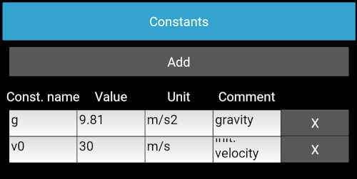
Const. name (mandatory): Name of the constant (as to be used in the equation).
Value (mandatory): Value of the constant. This can be either a simple value - e.g. ‘2.5’ - or python expression - e.g. ‘np.pi / 2’
Unit (optional): A unit for the constant - e.g. ‘kg’. This unit will only be used as a label in the plot title.
Comment (optional): A comment - e.g. to explain the meaning of the constant like ‘gravity’. This comment will be added as comment line in the python script file, if you export the project via the ‘Export’ button.

Plotting curve sets¶

If you want to create curve sets you can specify one constant as a curve set constant in the ‘Curve set parameters’ section. simple-plotter provides two ways of defining curve set values:

in terms of a defined number of equidistant values between a min., max. value

as a list of explicitly defined values

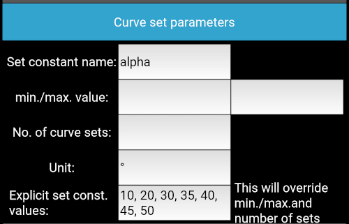
You can define following properties:

Set constant name (mandatory): Name of the constant (as to be used in the equation).
min./max. value (mandatory, if no explicit values are defined): Limits of automatically generated values - requires no. of curve sets to be defined as well
No of. curve sets (mandatory, if no explicit values are defined): Number of sets values to generate - requires min. and max. value to be defined as well
Unit (optional): A unit for the set constant. Will be displayed in the plot legend with each set value
Explicit set const. values (mandatory, if min./max. and/or number of curve sets not defined): A comma separated list of explicit values. If this is defined the definition of min./max. and no. of curve sets will be ignored. If you want to switch back to min./max. definition just delete all text in this field.

Plot labels¶

You can define some plot annotations in the ‘Plot labels’ section.

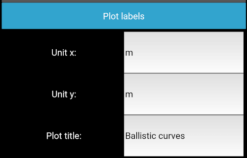
Unit x (optional): Appends a unit to the variable name on the x-axis
Unit y (optional): Appends a unit to the variable name on the y-axis
Plot title (optional): A user defined title to display above the plot. If this is empty or ‘None’ a plot title will automatically be generated from the function name, variable name, equation and defined constants - e.g. ‘f(x)=a*x**2+b*x, a=3.0, b=5.0’

Load, save and export¶

With the ‘Save’ button you can save your current project - i.e. the equation definition and additional parameters to a file and restore it via the ‘Load’ button.

The ‘Export’ button will export a python script, which can be run as a standalone script to create the plot.

Note

You cannot recreate the project from an exported python script (created via the ‘Export’ button). To restore your project in simple-plotter use the ‘Save’ button to save a project file.

Advanced usage¶

This chapter describes how the input file format is structured and how the CLI version of simple-plotter can be used to generate python code files.

File format¶

The input file for simple-plotter is a JSON file. See an example below:

{
    "file_format_version": "1.0",
    "export_csv": false,
    "formula": {
        "constants": [
            {
                "Comment": "",
                "Unit": "",
                "Value": "2",
                "Const. name": "amp"
            }
        ],
        "equation": "amp * np.sin(2* freq * np.pi * t)",
        "explicit_set_values": "None",
        "function_name": "y",
        "function_unit": "",
        "no_sets": "5",
        "set_max_val": "5",
        "set_min_val": "1",
        "set_var_name": "freq",
        "set_var_unit": "Hz",
        "var_name": "t",
        "var_unit": "s"
    },
    "plot_data": {
        "end_val": "1",
        "grid": true,
        "no_pts": "500",
        "plot_title": "",
        "start_val": "0",
        "swap_xy": false,
        "user_data": [],
        "x_log": false,
        "y_log": false,
        "y_max": "None",
        "y_min": "None"
    }
}

The file content can be divided into 3 parts:

General information: The file_format_version identifies the version of the file format and is used to correctly parse the information TODO: add JSON schema for different versions export_csv is intended for future use - currently this value has no effect.
formula: This part contains all information, which defines the mathematical problem - e.g. the equation, constants, unit, etc. For details see the explanations on these properties above.
plot_data: This part contains all information, which define the appearance of the plot - e.g. start and values for x- and y-axis, lin. or log. scale, etc. For details see the explanations on these properties above.

CLI usage¶

The basic syntax to run the CLI tool is:

simple-plotter [options] -i <input_file_name>

Where following options are available:

--help: Displays a help screen
--input or -i: This is the only mandatory option, which must be followed by the JSON input file name
--output or -o: If this option including an output file name (e.g. -o output.py) is set, the generated code will be saved to the corresponding file. If this option is omitted the code will just be printed to the terminal.
--plotlib or -p: This option defines, which plotting library shall be used. Currently ‘matplotlib’ and ‘kivy-graden/graph’ are supported. If this option is omitted the code will be generated for matplotlib.
--no-check or -n: This option disables the code checker. It is not recommended to use this option. If it is not checked the code checker will analyse the code for errors and illegal statements (e.g. un-allowed function calls) and thus provides some basic security.

Running the CLI tool on the example above (which can also be found as sine_waves.json in the examples folder in source code repository) with following command will create a python script with code for a kivy-garden/graph plot and save it to ‘test.py’ file.

simple-plotter --plotlib kivy-garden/graph -i ./simple_plotter/examples/sine_waves.json -o test.py

The content of the ‘test.py’ code file is shown below:

# this code has been auto-generated by simple_plotter
import numpy as np

import simple_plotter.core.advanced_graph as kv_graph

# function definition
def f(t, freq, amp):
    return amp * np.sin(2* freq * np.pi * t)

# definition of constants
amp = 2

# variable definition
t = np.linspace(0, 1, num=500)

# set constants definition
freq = np.linspace(1, 5, 5)
y = f(t, freq[0], amp)

# plot setup
graph = kv_graph.AnnotatedLinePlot(xlabel="t [s]",
    ylabel="y",
    y_grid_label=True, x_grid_label=True, padding=5,
    x_grid=True, y_grid= True, xlog=False, ylog=False
    , title="y(t)=amp * np.sin(2* freq * np.pi * t), amp = 2"
)
for set_const in freq:
    results = f(t, set_const, amp)
    graph.plot(t, results, label="freq="+str(set_const)+" [Hz]")



# uncomment the code below, if you want run this as a standalone script
# from kivy.app import App
#
# class Plot(App):
#
#     def __init__(self):
#         super().__init__()
#
#     def build(self):
#         return graph
#
# Plot().run()

As can be seen the code to actually create the plot is out-commented. If you want to run this script to generate a standalone plot, you should un-comment the lines at the end of the script before you run it.